Is rectified flow theoretically better than Diffusion Model? How to "cook" a good diffusion model in practice?
April 20, 2025 by Jiachen
When considering the task of generating images from Gaussian noise, the answer is No, meaning that diffusion models could also reach SOTA performance with carefully designed components.
Key Takeaways:
- The or prediction parameterization amplifies the diffusion model prediction error during sampling and is inferior in maintaining model training robustness. In contrast, the velocity prediction in rectified flow provides better training dynamics, making the training more robust thus further reducing the gap between the exact minimum of the mean-squared optimization objective and the approximated model prediction .
- To enhance model generation quality with the least inference cost, we should pay much attention to the designs of diffusion model, including the forward SDE, pre-conditioning, training objective (loss weighting and noise level sampling), reverse ODE, numerical solver and time steps . But, in practice, if you're new to image generation,
Section 1: Basics of DM and RF
Let's first revisit the mathmatical details of diffusion model and rectified flow. If you are familiar with them, feel free to jump to Section 2. Otherwise, you could also refer to the other blogs that introduces rectified flow and diffusion models in detail.
Diffusion Model
A diffusion model[1,2] is mathematically defined by the forward SDE, which can be written as:
where is a vector-valued function known as the drift coefficient of , is a scalar function known as the diffusion coefficient of , and is the standard Wiener process. When sampling along the forward process, we could generate a series of samples indexed by a continous time variable , such that and . is the target data distribution for which we have i.i.d samples for training our model, while is commonly chosen as a Gaussian distribution .
Given the forward SDE, we have the corresponding reverse SDE that starts from to .
Here, is the standard Wiener process when time flow backwards from to . is an infinitesimal negative timestep. denotes the probability distribution of sample at time step . As a result, given the score function at time step , we can sample along the reverse process and simulate to generate data from .
The score function can be approximated by the following score matching objective:
where is a weighting funciton, is uniformly sampled over , , , which denotes the transition kernel from to . It has the general form:
where
where we assume a linear structured drift coefficient: .
Given the definition of the transition kernel, the score of the conditional distribution can be decomposed as:
In practice, we typically parameterize the score model as -prediction or -prediction. Namely: or .
For brevity, we consider the diffusion model defined in EDM, where and , , and . As a result, we have and . The -prediction and -prediction parameterization can be written as: and respectively.
Rectified FLow
Rather than starting from SDE training to ODE sampling as in diffusion models, the rectified flow[4] proposes approximating a forward ODE with a velocity model . The forward ODE is defined as
where , , . The above ODE moves sample from to in . To transport backwards from to , it proposes to approximate an ODE that yields the same marginal distribution of as the above equation. The training objective is
Section 2: What's the difference between DM and RF? The training dynamics
When parameterizing the score model with the - or -prediction, the model is dictated to predict the noise or at time step . Considering that these two parameterizations only result in different optimization weight coefficient, without loss of generality, let's focus on analyzing the weakness of the -prediction formulation. With the -prediction model parameterization, the signal is reconstructed via . This leads to the model prediction eror being magnified by a factor of , which introduces excessive error during early sampling process and results in poor sample generation quality in particular when the total number of discretization step is small.
In contrast, RFs train , , to predict the velocity . During sampling, we traverse backwards in time step-by-step via:
Although the model prediction is also multiplied by a coefficient , the prediction error remains constrained. This is because ranges in in RFs. In addition, the RFs' training velocity objective also provides a practically better training dynamics by making the training more robust, reducing unexpected prediction error made by . To demonstrate this, we decompose the training objective in Equation 2 at time into a irreducible constant error and approximation error:
The irreducible constant error is the lower bound of the optimization objective at time while the approximation error determines how good the model performs. An optimal training dynamics largely benefits model convergence and pushes the approximation error to lower values. The analysis on the decomposed training objective is also applicable to diffusion models, where the optimal solution for Equation 1 is . We refer readers to Figure 5 in FasterDiT[5] for more empirical evidence on this.
For diffusion model, to mitigate model prediction error during training and bring it under control during sampling, it's more reasonable to predict the expected signal directly at large . As a result, EDM proposes to predict a mixture of noise and clean image at different . Specifically, it parameterizes the score model as:
where and is the scalar function. The training objective becomes:
As demonstrated in Figure 1, for and are chosen such that the variance of effective target equals to 1: . Besides, when , , predicts signal ; when , , predicts . The above design ensures the model prediction error is amplified as little as possible across all time steps. By adopting the parameterization and preconditioning, the training is more stable and robust, as evidenced by the experiments (Table 2) in EDM[3].

Is RF preferrable due to a straight sampling trajectory? No
One mistaken concept of RF is its learned sampling trajectory is "straight", leading to a faster sampling and better generation perforamnce. However, this is wrong. RF is preferred in many scenarios primarily due to its simpler and more concise implementations. When training DMs, in particular DDPM, one should write forward and reverse sampling functions, computing the drift and diffusion coefficients and the posterior mean. The implementation details are notoriously tedious yet largely impact the final generation performance. While for RF, the forward and sampling is simple and staightfoward.
Here, we discuss one toy example to compare the learned sampling trajectories of RF and DM. Consider target data distribution , RF sampling relies the velocity function , which has analytical solution in this scenario. Recall that Take posterior expectation with respect to on both sides, we have:
Here, . Besides, . By substituting it into Eq 3, we have:
With Tweedie's formula, the clean image is , thus we could compute the posterior mean by:
, Therefore, we have:
By setting , we could plot its sampling trajectory in Fig 2. Similarly, we could derive the score function thus the analytic solution of EDM's ODE sampling function (described above).
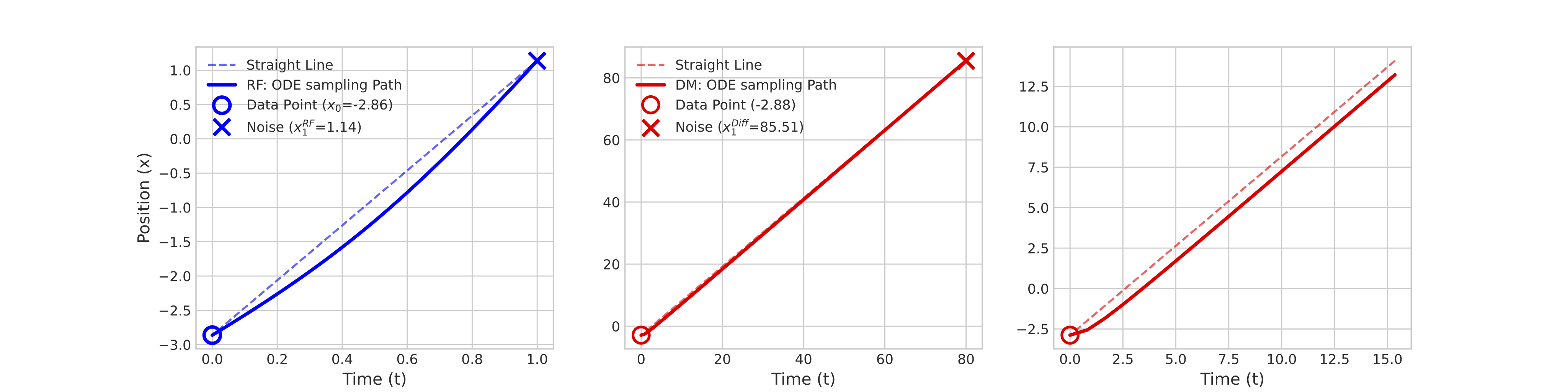
In the above examples, an interesting observation is that both sampling trajectories of diffusion model and flow model have a liner-nonlinear-linear structure. In [], the authors discuss this phenomenon within the context of diffusion model. They point out that the high-dimensional trajectories can be well-represented by a 3D sub-space. This is because each trajectory exhibits a very small deviation from the straight line joining its beginning (initial noise) and end points (denoised output). As a result, in the 3D sub-space, the trajectory shows a "boomerange" shape.
Section 3: How to train a diffusion model?
Given the above analysis, the model prediction error plays a key role in the generation peformance. Besides, the ODE solver and curvature of sampling trajectory are also important factors that affect model performance especially when the total number of discretization step is limited. To improve the sampling quality of DMs, the following aspects require careful designs, including:
- Choice of the diffuison forward process, which defines the PF-ODE sampling trajectory. A less curved sampling trajectory naturally supports larger discretization time step size. However, even when approximating the score with a sub-optimally designed SDE, we could generate samples by utilizing a different yet largely improved ODE, such as setting and as done in EDM[3].
- Preconditioning, loss weighting, and noise level sampling, which dictates training dynamics and the model prediction errors. A better training objective lowers model prediction errors and make the training more robust.
- SDE/ODE solver and time discretization schedule. The numerical solver introduces truncation error related to the curvature of the sampling trajectory and the time discretization schedule determines how the truncation error are distributed among different noise levels. The step size should decrease monotonically with decreasing .
Reference
[1] Denoising diffusion probabilistic models.
[2] Score-based generative modeling through stochastic differential equations.
[3] Elucidating the design space of diffusion-based generative models.
[4] Flow straight and fast: Learning to generate and transfer data with rectified flow.
[5] FasterDiT: Towards Faster Diffusion Transformers Training without Architecture Modification
[6] On the Trajectory of ODE-based Diffusion Sampling.